EIE: Efficient Inference Engine on Compressed Deep Neural Network

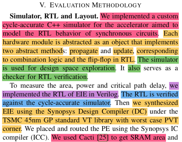
EIE.pdf: https://www.cs.virginia.edu/~smk9u/CS6501F16/p243-han.pdf

Note: This post covers part of 'Evaluation Section', but I may separate 'Evaluation Section' into another post.

Let's start from AlexNet

(figure from: Analysis of Sparse Convolutional Neural Networks
  http://ece757.ece.wisc.edu/project_talks/sparse.pptx)

// AlexNet Layers in text.
  %conv1_1 = Conv(%data_0, %conv1_w_0, %conv1_b_0)
  %conv1_2 = Relu(%conv1_1)
  %norm1_1 = LRN(%conv1_2)
  %pool1_1 = MaxPool(%norm1_1)
  %conv2_1 = Conv(%pool1_1, %conv2_w_0, %conv2_b_0)
  %conv2_2 = Relu(%conv2_1)
  %norm2_1 = LRN(%conv2_2)
  %pool2_1 = MaxPool(%norm2_1)
  %conv3_1 = Conv(%pool2_1, %conv3_w_0, %conv3_b_0)
  %conv3_2 = Relu(%conv3_1)
  %conv4_1 = Conv(%conv3_2, %conv4_w_0, %conv4_b_0)
  %conv4_2 = Relu(%conv4_1)
  %conv5_1 = Conv(%conv4_2, %conv5_w_0, %conv5_b_0)
  %conv5_2 = Relu(%conv5_1)
  %pool5_1 = MaxPool(%conv5_2)
  %fc6_1 = Gemm(%pool5_1, %fc6_w_0, %fc6_b_0)
  %fc6_2 = Relu(%fc6_1)
  %fc6_3, %_fc6_mask_1 = Dropout(%fc6_2)
  %fc7_1 = Gemm(%fc6_3, %fc7_w_0, %fc7_b_0)
  %fc7_2 = Relu(%fc7_1)
  %fc7_3, %_fc7_mask_1 = Dropout(%fc7_2)
  %fc8_1 = Gemm(%fc7_3, %fc8_w_0, %fc8_b_0)
  %prob_1 = Softmax(%fc8_1)
  return %prob_1

The parameters size of AlexNet is 240 MB, FC6 weights (fc6_w_0) contribute 144 MB, FC7 weights (fc7_w_0) contribute 64 MB. 

The weight has to be put in DRAM, and access DRAM is costly in terms of cycle time and energy.

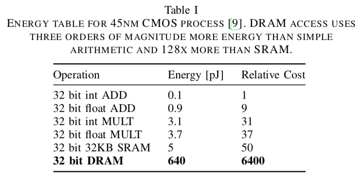
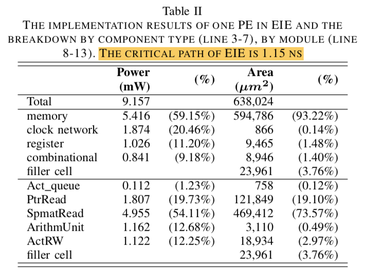
Table from EIE paper.

It's a heavy burden for power and performance constrained embedded devices, so, Professor Han et al. presented methodology DEEP COMPRESSION to compress deep neural network without loss of accuracy. The result is very impressive:



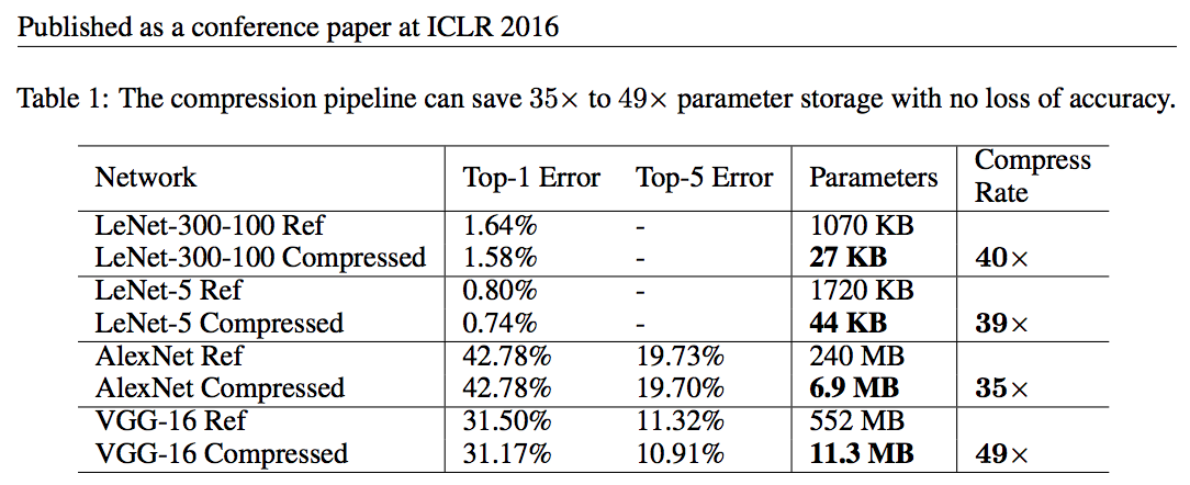
For AlexNet:

• Original: 240 MB
• Compressed: 6.9 MB (included the meta-data for sparse representation)
  => 35 Times Compress rate

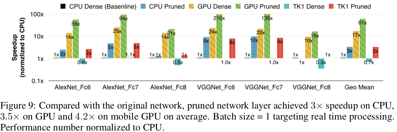
Performance: (DEEP COMPRESSION Figure 9)


Energy: (DEEP COMPRESSION Figure 10)

It gets very good performance in execution time and energy efficiency. In order to more efficiently operate on compressed model, Professor Han et al. proposed EIE (Efficient Inference Engine).


What is EIE?

• A specialized accelerator that performs customized sparse matrix vector multiplication
• A scalable array of processing elements (PEs)

Each PE

• Holds 131K weights of the compressed model
• Perform 800 million weight calculations per second
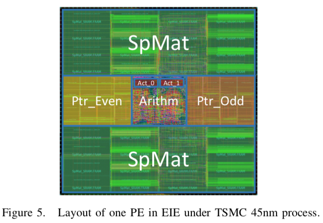
• In 45nm CMOS:
• area = 0.638mm2
• dissipates = 9.16mW at 800MHz

Focus on Matrix-vector multiplication (M×V), Why?

• Convolutional neural network (CNN)
• Fully Connected layers are implemented with M×V
• In object detection algorithms fast R-CNN (Girshick, 2015),  38% computation time is consumed on FC layers on uncompressed model
• Recurrent neural network (RNN)
• M×V operations are performed on the new input and the hidden state at each time step, producing a new hidden state and the output.
• Long-Short-Term-Memory (LSTM)
• A widely used structure of RNN cell
• Each LSTM cell can be decomposed into eight M×V operations
• Widely used in image captioning, speech recognition and natural language processing

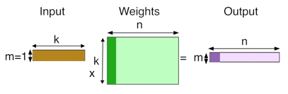
Fully Connected layer

• Fully Connected Layers form the final layers of a typical CNN and implemented as Matrix Vector Multiply operation. (GEMV).

(Text and figure from: Analysis of Sparse Convolutional Neural Networks

  http://ece757.ece.wisc.edu/project_talks/sparse.pptx)

M×V Computation, e.g. AlexNet and VGG-16

• (Original) Uncompressed (Dense) Model
  
• a is the input activation vector, b is the output activation vector, W is the weight matrix

• Deep Compression (Sparse) Model
  
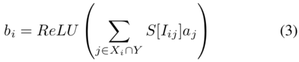
• Weight sharing replaces each weight Wij with a four-bit index Iij into a shared table S of 16 possible weight values.
• Xi represents the static sparsity of W
• Y represents the dynamic sparsity of a
• EIE perform the indexing S [Iij ] and the multiply-add only for non-zero of Wij and aj

EIE on Compressed sparse column (CSC) format, use figure 2 (4 PEs configuration) as an example

• PE0 holds:
• rows W0, W4, W8, W12 of Matrix W 
• a0, a4 of input activations
• b0 , b4 , b8 of output activations
  => Given PEk, PEk holds Wi, ai, bi for which i (mod N) = k.

• Figure 3. Memory layout, use PE0 as an example
• Virtual Weight: contains the non-zero weights
• Relative Row Index:
• Same length as Virtual Weight
• Encodes the number of zeros before the corresponding entry in Virtual Weight
• Each entry is represented by a four-bit value
• If more than 15 zeros appear before a non-zero entry we add a zero in Virtual Weight
• E.g. [0,0,1,2,0,0,0,0,0,0,0,0,0,0,0,0,0,0,0,0,0,0,3]
• Virtual Weight = [1,2,0,3]
• Relative Row Index = [2,0,15,2] 
• Column Pointer
• Pointing to the beginning of the vector for each column
• Column Pointer[0] = 0, column 0's beginning = Virtual Weight [0]
• Column Pointer[1] = 3, column 1's beginning = Virtual Weight [3]
• Column Pointer[2] = 4, column 2's beginning = Virtual Weight [4]
• ...
• Column Pointer[7] = 11, column 7's beginning = Virtual Weight [11]
• Column Pointer[8] = 13
• final entry in Column Pointer points one beyond the last vector element
• the number of non-zeros in column j (including padded zeros) is given by pj+1 − pj.

• Multiplication, use figure 2 as an example.
• Scan input activations a
• a2 is not zero, broadcast value a2 and column index 2 to all PEs
• PE0 multiplies a2 by W0,2 and W12,2
• PE1 has all zeros in column 2
• PE2 multiplies a2 by W2,2 and W14,2
• PE3 multiplies a2 by W11,2 and W15,2
• And so on ..

• This process may suffer load imbalance because each PE may have a different number of non-zeros in a particular column.
• Can be reduced by queuing.

EIE Hardware Implementation

• Central Control Unit (CCU)
• Controls an array of PEs
• Receives non-zero input activations from a distributed Leading Non-zero Detection network and broadcasts these to the PEs
• Communicates with the host
• Activation Queue (Act Queue)
• Get Non-zero element aj and index j from queue (pushed by CCU)
• Pointer Read Unit
• Index j is used to look up the start and end pointers pj and pj+1
• Store pointers in two single-ported SRAM banks for one cycle access
• Pointers are 16-bits in length.
• Sparse Matrix Read Unit
• Each entry in the SRAM is 8-bits
• 4-bit for Virtual Weight, 4-bit for Relative Row Index
• For efficiency (see paper Section VI) the PE’s slice of encoded sparse matrix I is stored in a 64-bit-wide SRAM
  => fetch 8 entry a time
• Arithmetic Unit
• Decode 4-bit Virtual Weight to a 16-bit fixed-point number via a table look up
• Use Relative Row Index to index an accumulator array (the destination activation registers) 
• A bypass path
• if the same accumulator is selected on two adjacent cycles.
• Activation Read/Write
• Two activation register files for source and destination
• The role of source and destination is exchanged in next layer
  => no additional data transfer is needed to support multi-layer feed-forward computation
•  Distributed Leading Non-Zero Detection
• Each group of 4 PEs does a local leading non-zero detection on their input activation. The result is sent to a Leading Non-zero Detection Node (LNZD Node)
• Each LNZD node finds the next non-zero activation across its four children and sends this result up the quadtree
• At the root LNZD Node, the selected non-zero activation is broadcast back to all the PEs via a separate wire placed in an H-tree

Evaluation